data-lakehouse-iceberg-trino-spark
|
This demo shows a data workload with real world data volumes and uses significant amount of resources to ensure acceptable response times. It will most likely not run on your workstation. There is also the smaller trino-iceberg demo focusing on the abilities a lakehouse using Apache Iceberg offers.
The The demo was developed and tested on a kubernetes cluster with 10 nodes (4 cores (8 threads), 20GB RAM and 30GB HDD). Instance types that loosely correspond to this on the Hyperscalers are:
In addition to these nodes the operators will request multiple persistent volumes with a total capacity of about 1TB. |
|
This guide assumes that you already have the demo |
This demo will
-
Install the required Stackable operators
-
Spin up the following data products
-
Trino: A fast distributed SQL query engine for big data analytics that helps you explore your data universe. This demo uses it to enable SQL access to the data
-
Apache Spark: A multi-language engine for executing data engineering, data science, and machine learning. This demo uses it to stream data from Kafka into the lakehouse
-
MinIO: A S3 compatible object store. This demo uses it as persistent storage to store all the data used
-
Apache Kafka: A distributed event streaming platform for high-performance data pipelines, streaming analytics and data integration. This demos uses it as an event streaming platform to stream the data in near real-time
-
Apache NiFi: An easy-to-use, powerful system to process and distribute data. This demos uses it to fetch multiple online real-time data sources and ingest it into Kafka
-
Apache Hive metastore: A service that stores metadata related to Apache Hive and other services. This demo uses it as metadata storage for Trino and Spark
-
Open policy agent (OPA): An open source, general-purpose policy engine that unifies policy enforcement across the stack. This demo uses it as the authorizer for Trino, which decides which user is able to query which data.
-
Apache Superset: A modern data exploration and visualization platform. This demo utilizes Superset to retrieve data from Trino via SQL queries and build dashboards on top of that data
-
-
Copy multiple data sources in CSV and Parquet format into the S3 staging area
-
Let Trino copy the data from staging area into the lakehouse area. During the copy transformations such as validating, casting, parsing timestamps and enriching the data by joining lookup-tables are done
-
Simultaneously start a NiFi workflow, which fetches datasets in real-time via the internet and ingests the data as JSON records into Kafka
-
Spark structured streaming job is started, which streams the data out of Kafka into the lakehouse
-
Create Superset dashboards for visualization of the different datasets
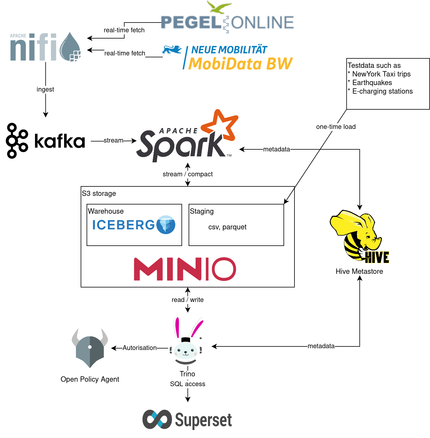
You can see the deployed products as well as their relationship in the following diagram:
Apache Iceberg
As Apache Iceberg states on their website:
Apache Iceberg is an open table format for huge analytic datasets. Iceberg adds tables to compute engines including Spark, Trino, PrestoDB, Flink, Hive and Impala using a high-performance table format that works just like a SQL table.
This demos uses Iceberg as it plays along nicely with object storage as well as having a Trino and Spark integration. In also provides the following benefits among other things over simply putting Apache Parquet files in S3 using the Hive connector:
-
Standardized specification how to store tables: Using this standardized specification multiple tools such as Trino, Spark and Flink and read and write Iceberg tables.
-
Versioned tables with snapshots, time travel and rollback mechanisms
-
Row level updates and deletes: Deletes will be written as separate files for best performance and will be compacted with the mechanism described below.
-
Built in compaction: It is recommended to run some table maintenance functions such as compacting smaller files (including delete files) into larger files for best query performance. Iceberg offers out-of-the-box tools for this.
-
Hidden partitioning: Image you have a table
sales (day varchar, ts timestamp)partitioned byday. Lot’s of times users would run a statement such asselect count(*) where ts > now() - interval 1 dayresulting in a full table scan as the partition columndaywas not filtered in the query. Iceberg resolves this problem by using hidden partitions. In Iceberg your table would look likesales (ts timestamp) with (partitioning = ARRAY['day(ts)']). The columndayis not needed anymore, and the queryselect count(\*) where ts > now() - interval 1 daywould use partition pruning as expected to only read one the partitions from today and yesterday.
If you want to read more on the motivation and the working principles on Iceberg, please have a read on there website or GitHub repo.
List deployed Stackable services
To list the installed installed Stackable services run the following command:
$ stackablectl services list --all-namespaces
 PRODUCT    NAME          NAMESPACE  ENDPOINTS                                          EXTRA INFOS

 hive       hive          default    hive                212.227.224.138:31022
                                     metrics             212.227.224.138:30459

 hive       hive-iceberg  default    hive                212.227.233.131:31511
                                     metrics             212.227.233.131:30003

 kafka      kafka         default    metrics             217.160.118.190:32160
                                     kafka               217.160.118.190:31736

 nifi       nifi          default    https               https://217.160.120.117:31499  Admin user: admin, password: adminadmin

 opa        opa           default    http                http://217.160.222.211:31767

 superset   superset      default    external-superset   http://212.227.233.47:32393    Admin user: admin, password: adminadmin

 trino      trino         default    coordinator-metrics 212.227.224.138:30610
                                     coordinator-https   https://212.227.224.138:30876

 zookeeper  zookeeper     default    zk                  212.227.224.138:32321

 minio      minio         default    http                http://217.160.222.211:32031   Third party service
console-http http://217.160.222.211:31429 Admin user: admin, password: adminadmin|
When a product instance has not finished starting yet, the service will have no endpoint. Starting all the product instances might take a considerable amount of time depending on your internet connectivity. In case the product is not ready yet a warning might be shown. |
MinIO
List buckets
The S3 provided by MinIO is used as persistent storage to store all the data used.
Open the minio endpoint console-http retrieved by stackablectl services list in your browser (http://217.160.222.211:31429 in this case).
Log in with the username admin and password adminadmin.
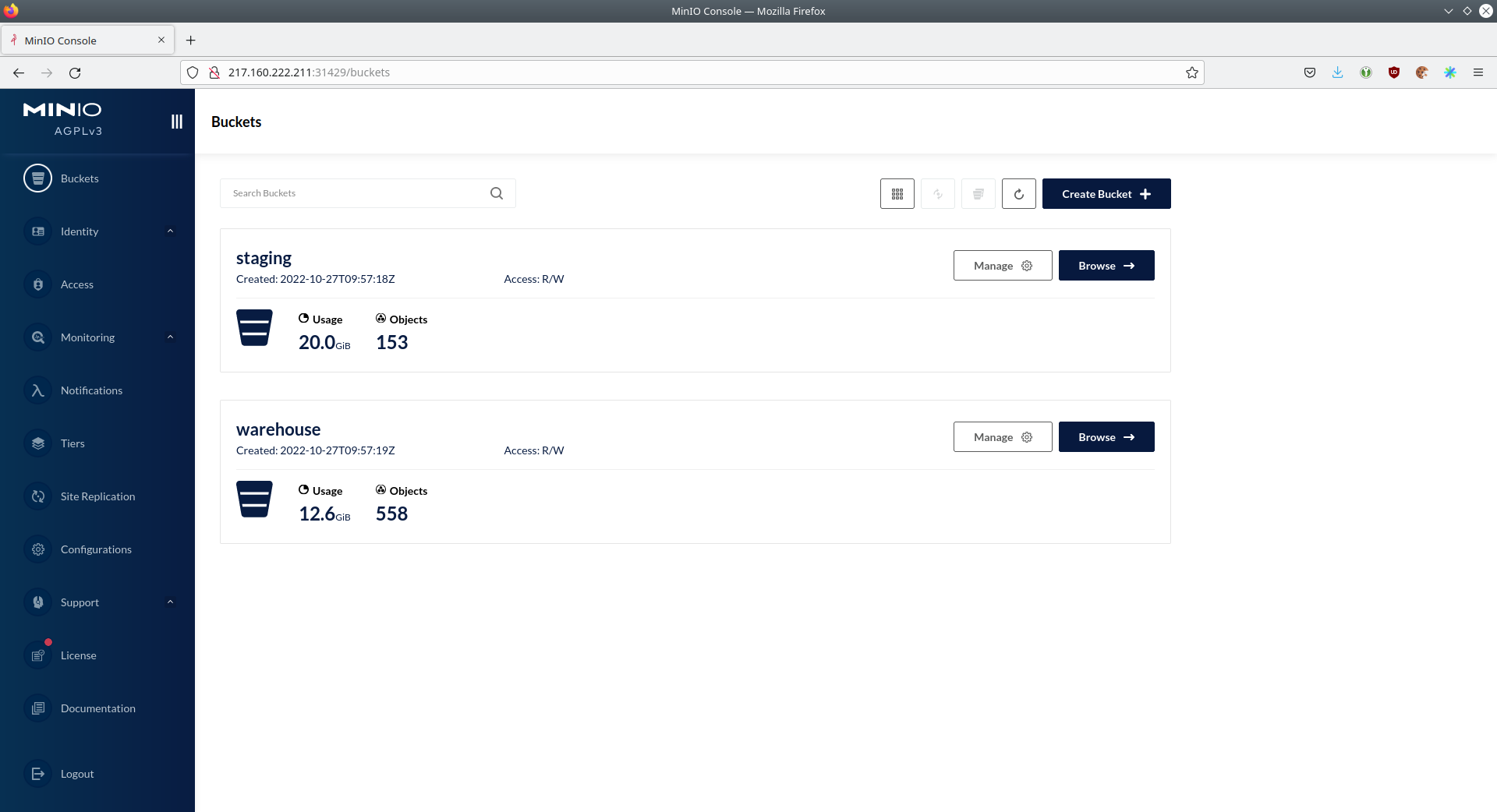
Here you can see the two buckets contained in the S3:
-
staging: The demo loads static datasets into this area. It is stored in different formats, such as CSV and Parquet. It does contain actual data tables as well as lookup tables. -
lakehouse: This bucket is where the cleaned and/or aggregated data resides. The data is stored in the Apache Iceberg table format.
Inspect lakehouse
Click on the blue button Browse on the bucket lakehouse.
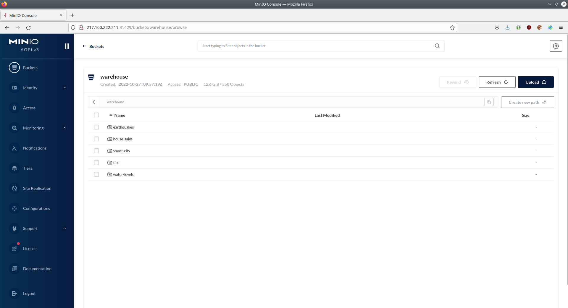
You can see multiple folders (called prefixes in S3) - each containing a different dataset.
Click on the folders house-sales afterwards the folder starting with house-sales-* afterwards 'data'.
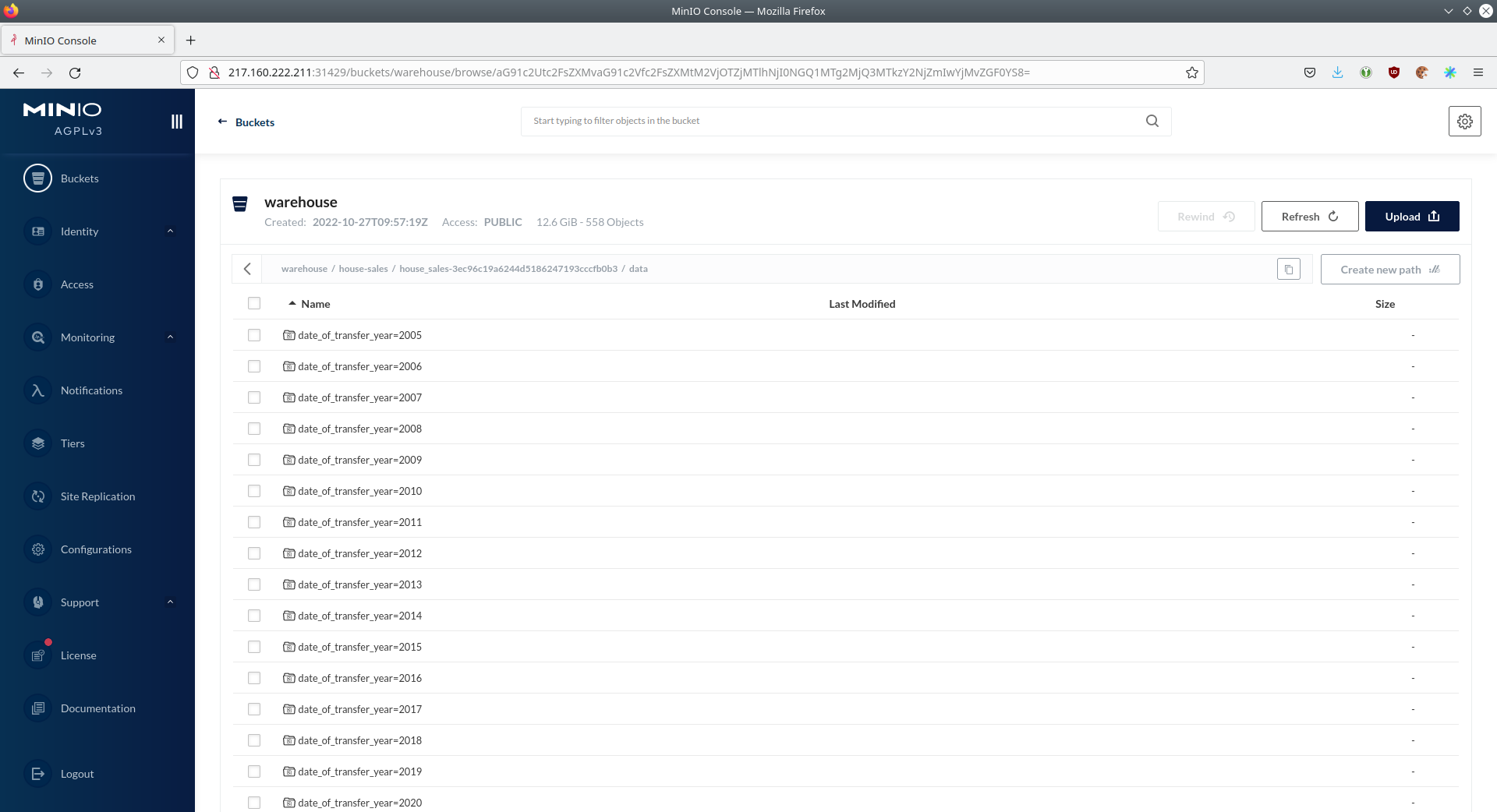
As you can see the table house-sales is partitioned by day.
Go ahead and click on any folder.

You can see that Trino has placed a single file here containing all the house sales of that particular year.
NiFi
NiFi is used to fetch multiple datasources from the internet and ingest it into Kafka near-realtime. Some data sources are statically downloaded (e.g. as CSV) and others are dynamically fetched via APIs such as REST APIs. This includes the following data sources:
-
Water level measurements in Germany (real-time)
-
Shared bikes in Germany (real-time)
-
House sales in UK (static)
-
Registered earthquakes worldwide (static)
-
E-charging stations in Germany (static)
-
NewYork taxi data (static)
View ingestion jobs
You can have a look at the ingestion job running in NiFi by opening the given nifi endpoint https from your stackablectl services list command output (https://217.160.120.117:31499 in this case).
If you get a warning regarding the self-signed certificate generated by the Secret Operator (e.g. Warning: Potential Security Risk Ahead), you have to tell your browser to trust the website and continue.
Log in with the username admin and password adminadmin.
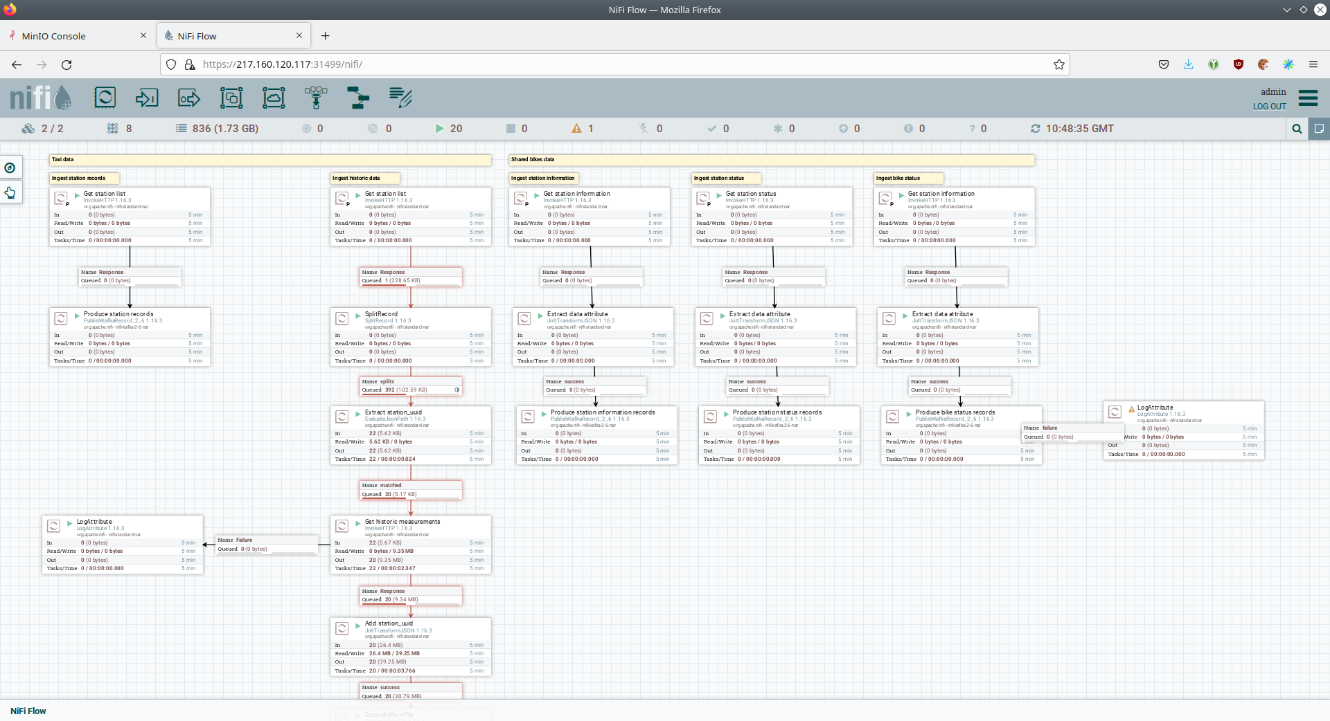
As you can see, the NiFi workflow consists of lots of components. You can zoom in by using your mouse and mouse wheel. On the left side are two strands, that
-
Fetch the list of known water-level stations and ingest them into Kafka
-
Continuously run a loop fetching the measurements of the last 30 for every measuring station and ingesting the measurements into Kafka
On the right side are three strands, that
-
Fetch the current shared bike stations information
-
Fetch the current shared bike stations status
-
Fetch the current shared bike bike status
For details on the NiFi workflow ingesting water-level data please read on the nifi-kafka-druid-water-level-data documentation on NiFi.
Spark
Spark Structured Streaming is used to stream data from Kafka into the lakehouse.
Access webinterface
To have access to the Spark WebUI you need to run the following command to port-forward the Port 4040 to your local machine
kubectl port-forward $(kubectl get pod -o name | grep 'spark-ingest-into-lakehouse-.*-driver') 4040Afterwards you can reach the Webinterface on http://localhost:4040.
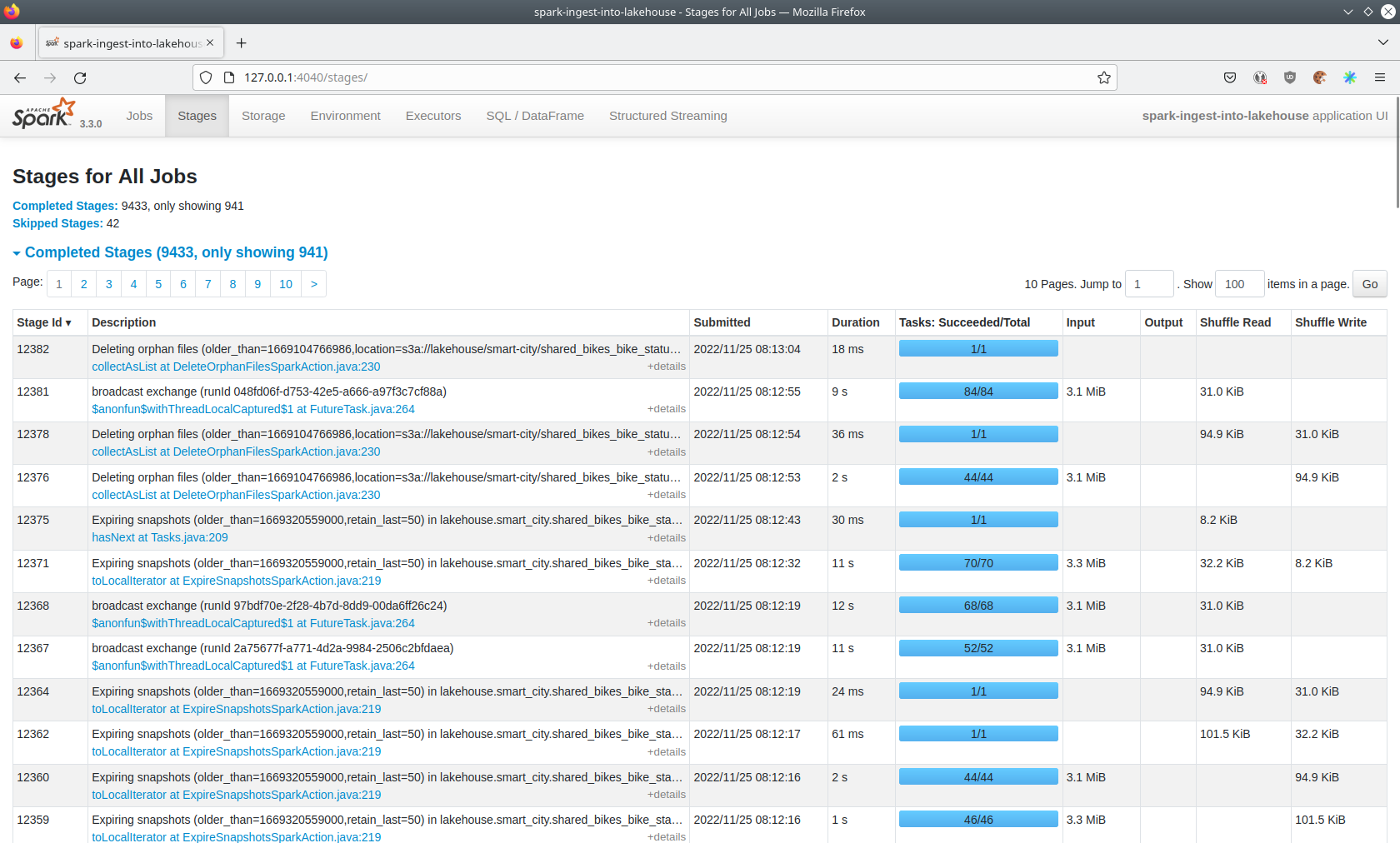
List running streaming jobs
On the UI the last jobs are shown. Each running Structured Streaming job creates lots of Spark jobs internally.
Click on the tab Structured Streaming to see the running streaming jobs.
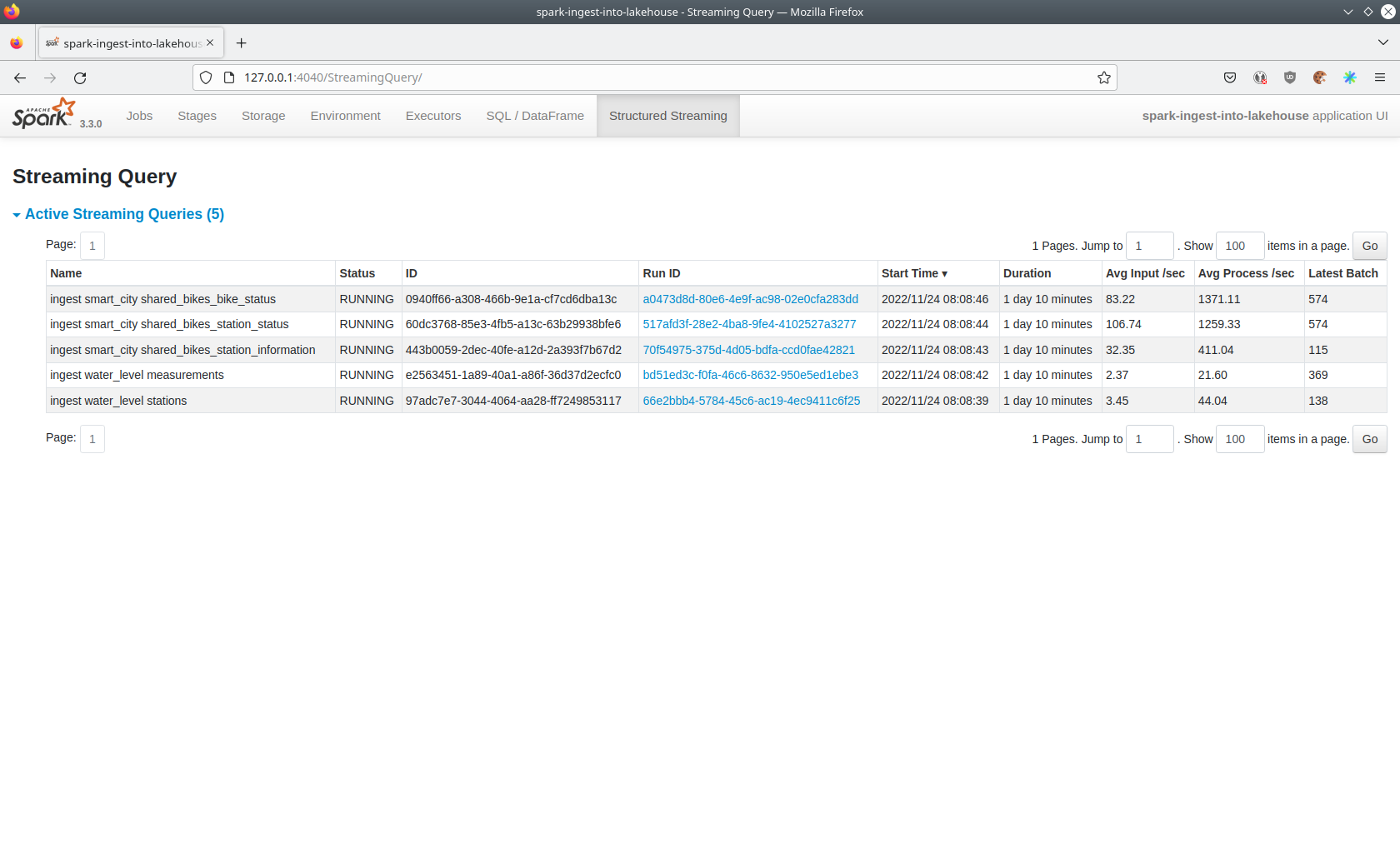
Five streaming jobs are currently running.
You can also click on a streaming job to get more details.
For the job ingest smart_city shared_bikes_station_status click on the Run ID highlighted in blue to open them up.
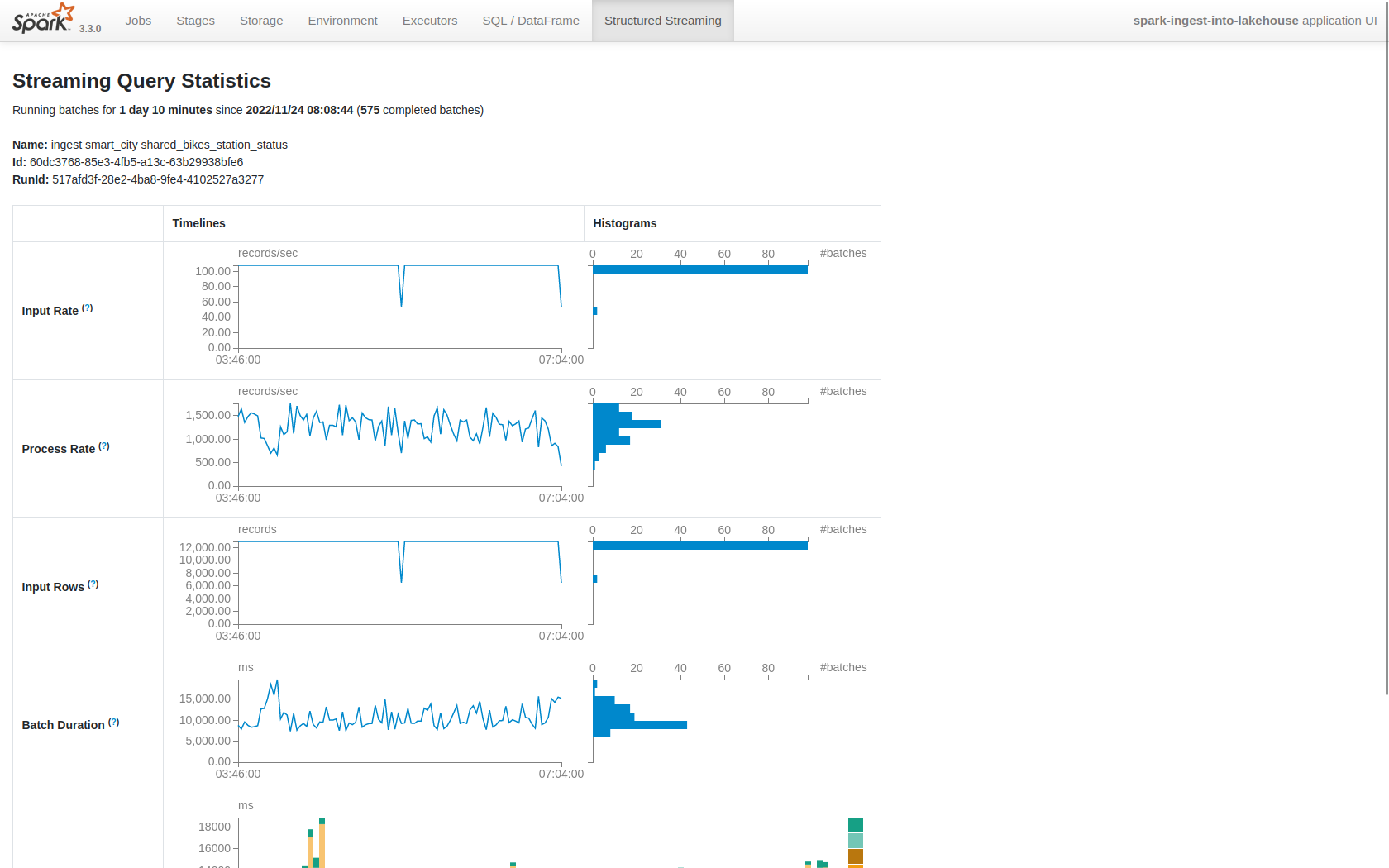
How the streaming jobs work
All the running streaming jobs have been started by the demo, to see the actual code submitted to Spark have a look in the demos code.
This document will explain one specific ingestion job - ingest water_level measurements.
The streaming job is written in Python using pyspark.
First off the schema used to parse the JSON coming from Kafka is defined.
Nested structures or arrays are supported as well.
This differs from job to job.
schema = StructType([ \
    StructField("station_uuid", StringType(), True), \
    StructField("timestamp", TimestampType(), True), \
    StructField("value", FloatType(), True), \
])
Afterwards, a streaming read from Kafka is started.
It reads from our Kafka at the address kafka:9092`and the topic called `water_levels_measurements.
When starting up the job will ready all the already existing messages in Kafka (read from earliest) and will process 50000000 records as a maximum in a single batch.
As the Kafka has a retention set up, Kafka records might alter out if the topic, before Spark has read the records.
This can be the case when the Spark application was shut down or crashed for too long.
In that case of this demo the streaming job should not error out.
For a production job failOnDataLoss should be set to true, so that missing data does not get unnoticed - and Kafka offsets need to be adjusted manually as well as maybe some post-loading of data.
Note: All of the following Python snippets belong to a single Python statement but are spilled into separate blocks for better explanation purposes.
spark \
.readStream \
.format("kafka") \
.option("kafka.bootstrap.servers", "kafka:9092") \
.option("subscribe", "water_levels_measurements") \
.option("startingOffsets", "earliest") \
.option("maxOffsetsPerTrigger", 50000000) \
.option("failOnDataLoss", "false") \
.load() \
So far we have a readStream reading from Kafka.
Records on Kafka are simply a byte-stream, so they must be converted to strings and the json needs to be parsed.
.selectExpr("cast(key as string)", "cast(value as string)") \
.withColumn("json", from_json(col("value"), schema)) \
Afterwards we only select the needed fields (coming from JSON).
We are not interested in all the other fields such as key, value, topic or offset.
If you are interested in the metadata of the Kafka records, such as topic, timestamp, partition and offset they are available as well.
Please have a look at the Spark streaming documentation on Kafka.
.select("json.station_uuid", "json.timestamp", "json.value") \After all this transformations we need to specify the sink of the stream, in this case the Iceberg lakehouse.
We are writing in the iceberg format using the update mode rather than the "normal" append mode.
Spark will aim for a microbatch every 2 minutes and will save it’s checkpoints (it’s current offsets on the Kafka topic) in the specified S3 location.
Afterwards the streaming job will be started by calling .start()
.writeStream \
.queryName("ingest water_level measurements") \
.format("iceberg") \
.foreachBatch(upsertWaterLevelsMeasurements) \
.outputMode("update") \
.trigger(processingTime='2 minutes') \
.option("checkpointLocation", "s3a://lakehouse/water-levels/checkpoints/measurements") \
.start()
Deduplication mechanism
One important part was skipped during the walkthrough:
.foreachBatch(upsertWaterLevelsMeasurements) \upsertWaterLevelsMeasurements is a Python function that describes how to insert the records coming from Kafka into the lakehouse table.
This specific streaming job removes all duplicate records, that can occur because of how the PegelOnline API works and gets called. As we don’t want duplicate rows in our lakehouse tables, we need to filter the duplicates out as follows.
def upsertWaterLevelsMeasurements(microBatchOutputDF, batchId):
    microBatchOutputDF.createOrReplaceTempView("waterLevelsMeasurementsUpserts")

    microBatchOutputDF._jdf.sparkSession().sql("""
    MERGE INTO lakehouse.water_levels.measurements as t
    USING (SELECT DISTINCT * FROM waterLevelsMeasurementsUpserts) as u
    ON u.station_uuid = t.station_uuid AND u.timestamp = t.timestamp
    WHEN NOT MATCHED THEN INSERT *
    """)
First of the dataframe containing the upserts (records coming from Kafka) will be registered as a temporary view, so they can be access via Spark SQL.
Afterwards the MERGE INTO statement is used to add the new records to the lakehouse table.
The incoming records are first de-duplicated (using SELECT DISTINCT * FROM waterLevelsMeasurementsUpserts), so that the data from Kafka does not contain duplicates.
Afterwards the - now duplication free - records get added to the lakehouse.water_levels.measurements, but only if they are not already present.
Upsert mechanism
The MERGE INTO statement can not only be used for de-duplicating data but also for updating existing rows in the lakehouse table.
The ingest water_level stations streaming job uses the following MERGE INTO statement:
MERGE INTO lakehouse.water_levels.stations as t
USING
    (
    SELECT station_uuid, number, short_name, long_name, km, agency, latitude, longitude, water_short_name, water_long_name
    FROM waterLevelsStationInformationUpserts
    WHERE (station_uuid, kafka_timestamp) IN (SELECT station_uuid, max(kafka_timestamp) FROM waterLevelsStationInformationUpserts GROUP BY station_uuid)
    ) as u
ON u.station_uuid = t.station_uuid
WHEN MATCHED THEN UPDATE SET *
WHEN NOT MATCHED THEN INSERT *
First of the data within a batch is de-deduplicated as well. The record containing station update with the highest Kafka timestamp is the freshest update and will be used during Upsert.
In case a record for a station (detected by the same station_uud) already exists, it’s contents will be updated.
In case the station is not known yet, it will be simply inserted.
The MERGE INTO also supports updating a subsets of fields and more complex calculation e.g. incrementing a counter.
For details have a look at the Iceberg MERGE INTO documentation.
Delete mechanism
The MERGE INTO statement also supports deleting rows from the lakehouse tables.
For details have a look at the Iceberg MERGE INTO documentation.
Table maintenance
As mentioned in the beginning, Iceberg supports out-of-the-box table maintenance such as compaction.
This demos executes some maintenance functions in a very basic Python loop with sleeps in between. For production the maintenance can be scheduled using Kubernetes CronJobs or using Apache Airflow, which is also supported by the Stackable Data Platform.
# key: table name
# value: compaction strategy
tables_to_compact = {
    "lakehouse.water_levels.stations": "",
    "lakehouse.water_levels.measurements": ", strategy => 'sort', sort_order => 'timestamp DESC NULLS LAST,station_uuid ASC NULLS LAST'",
    "lakehouse.smart_city.shared_bikes_station_information": "",
    "lakehouse.smart_city.shared_bikes_station_status": ", strategy => 'sort', sort_order => 'last_reported DESC NULLS LAST,station_id ASC NULLS LAST'",
    "lakehouse.smart_city.shared_bikes_bike_status": "",
}

while True:
    expire_before = (datetime.now() - timedelta(hours=12)).strftime("%Y-%m-%d %H:%M:%S")
    for table, table_compaction_strategy in tables_to_compact.items():
        print(f"[{table}] Expiring snapshots older than 12 hours ({expire_before})")
        spark.sql(f"CALL lakehouse.system.expire_snapshots(table => '{table}', older_than => TIMESTAMP '{expire_before}', retain_last => 50, stream_results => true)")

        print(f"[{table}] Removing orphaned files")
        spark.sql(f"CALL lakehouse.system.remove_orphan_files(table => '{table}')")

        print(f"[{table}] Starting compaction")
        spark.sql(f"CALL lakehouse.system.rewrite_data_files(table => '{table}'{table_compaction_strategy})")
        print(f"[{table}] Finished compaction")

    print("All tables compacted. Waiting 25min before scheduling next run...")
    time.sleep(25 * 60) # Assuming compaction takes 5 min run every 30 minutes
The scripts has a dictionary of all the tables to run maintenance on. The following procedures are run:
expire_snapshots
Each write/update/delete/upsert/compaction in Iceberg produces a new snapshot while keeping the old data and metadata around for snapshot isolation and time travel. The expire_snapshots procedure can be used to remove older snapshots and their files which are no longer needed.
remove_orphan_files
Used to remove files which are not referenced in any metadata files of an Iceberg table and can thus be considered “orphaned”.
rewrite_data_files
Iceberg tracks each data file in a table. More data files leads to more metadata stored in manifest files, and small data files causes an unnecessary amount of metadata and less efficient queries from file open costs. Iceberg can compact data files in parallel using Spark with the rewriteDataFiles action. This will combine small files into larger files to reduce metadata overhead and runtime file open cost.
Some tables will also be sorted during rewrite, please have a look at the documentation on rewrite_data_files.
Trino
Trino is used to enable SQL access to the data.
View WebUI
Open up the the given trino endpoint coordinator-https from your stackablectl services list command output (https://212.227.224.138:30876 in this case).
Log in with the username admin and password adminadmin.
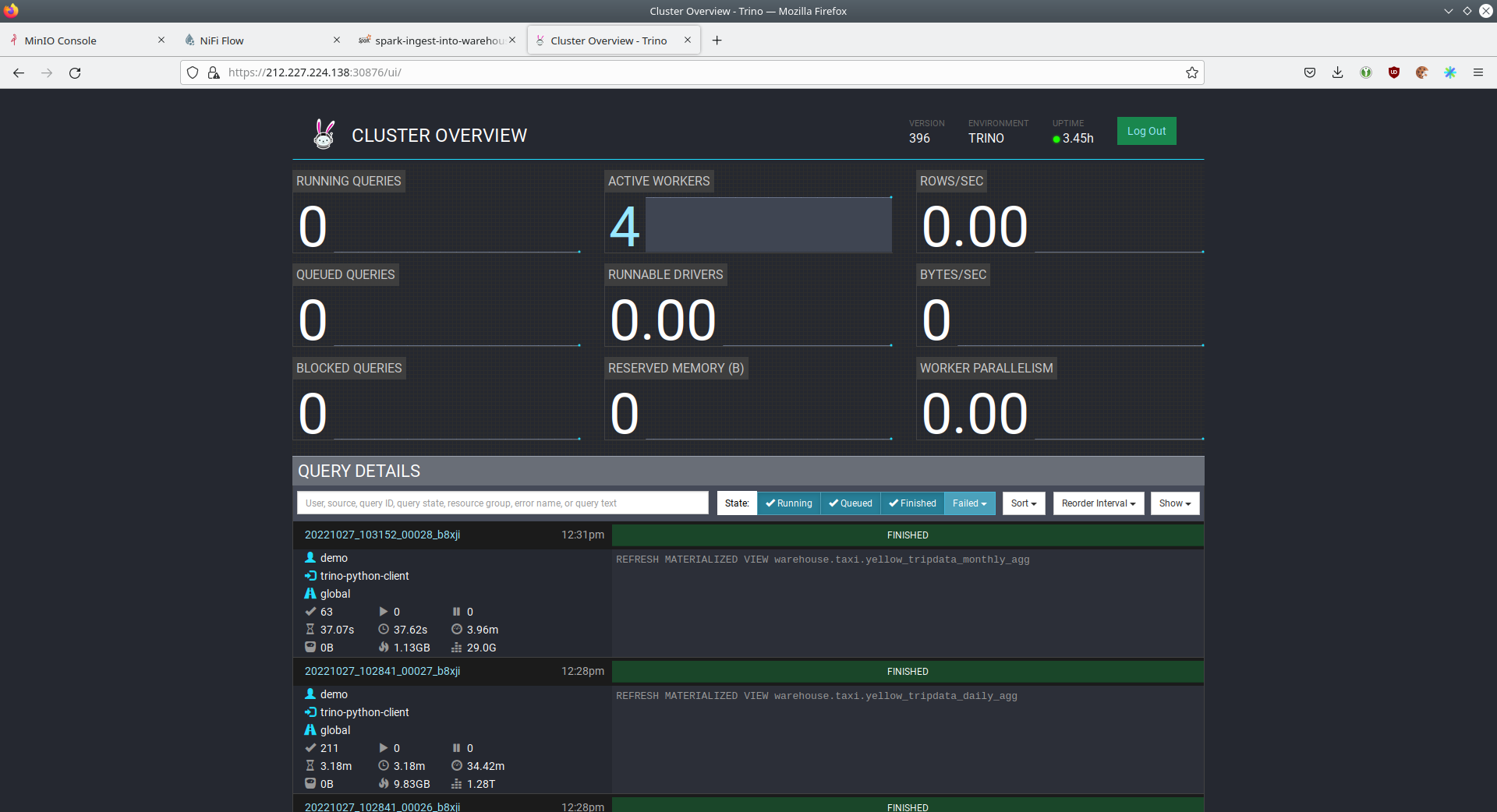
Connect with DBeaver
DBeaver is free multi-platform database tool that can be used to connect to Trino. Please have a look at the <TODO> trino-operator documentation on how to connect DBeaver to Trino.
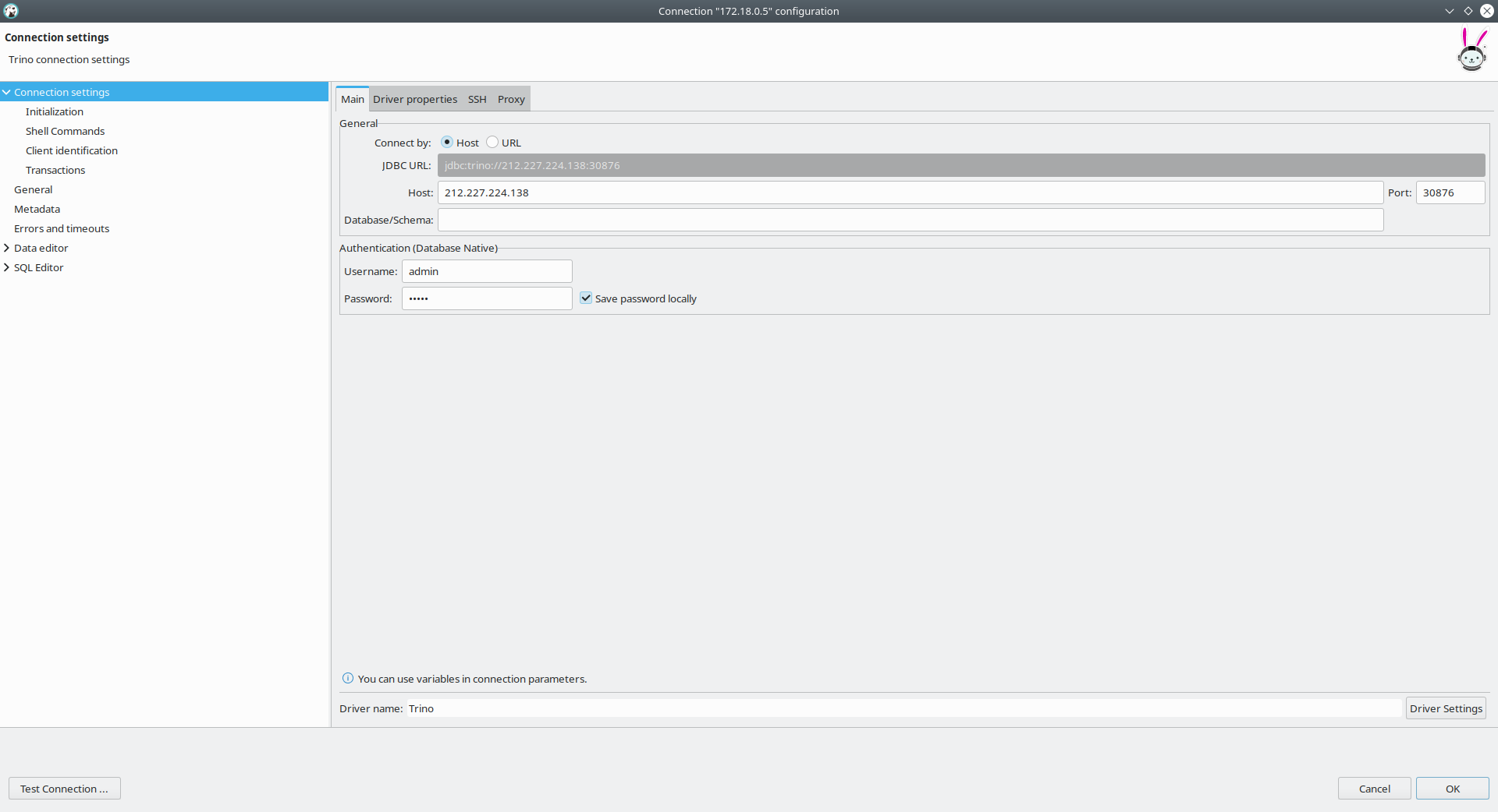
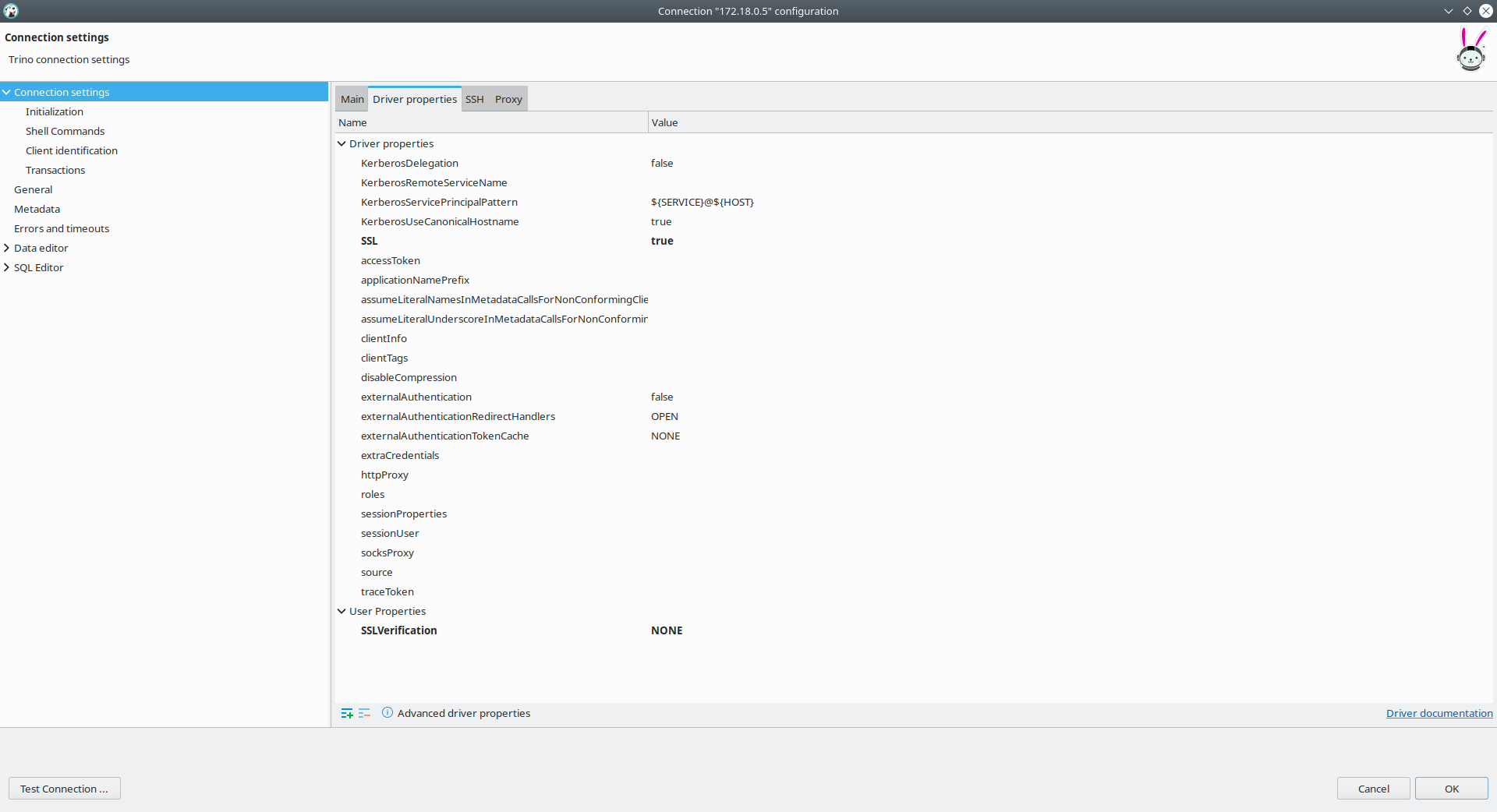
You need to modify the setting TLS to true.
Additionally you need to add the setting SSLVerification and set it to NONE.
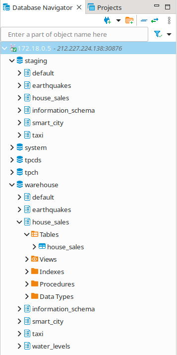
Here you can see all the available Trino catalogs.
-
staging: The staging area containing raw data in various data formats such as CSV or Parquet -
system: Internal catalog to retrieve Trino internals -
tpcds: TPCDS connector providing a set of schemas to support the TPC Benchmark™ DS -
tpch: TPCH connector providing a set of schemas to support the TPC Benchmark™ DS -
lakehouse: The lakehouse area containing the enriched and performant accessible data
Superset
Superset provides the ability to execute SQL queries and build dashboards.
Open the superset endpoint external-superset in your browser (http://212.227.233.47:32393 in this case).
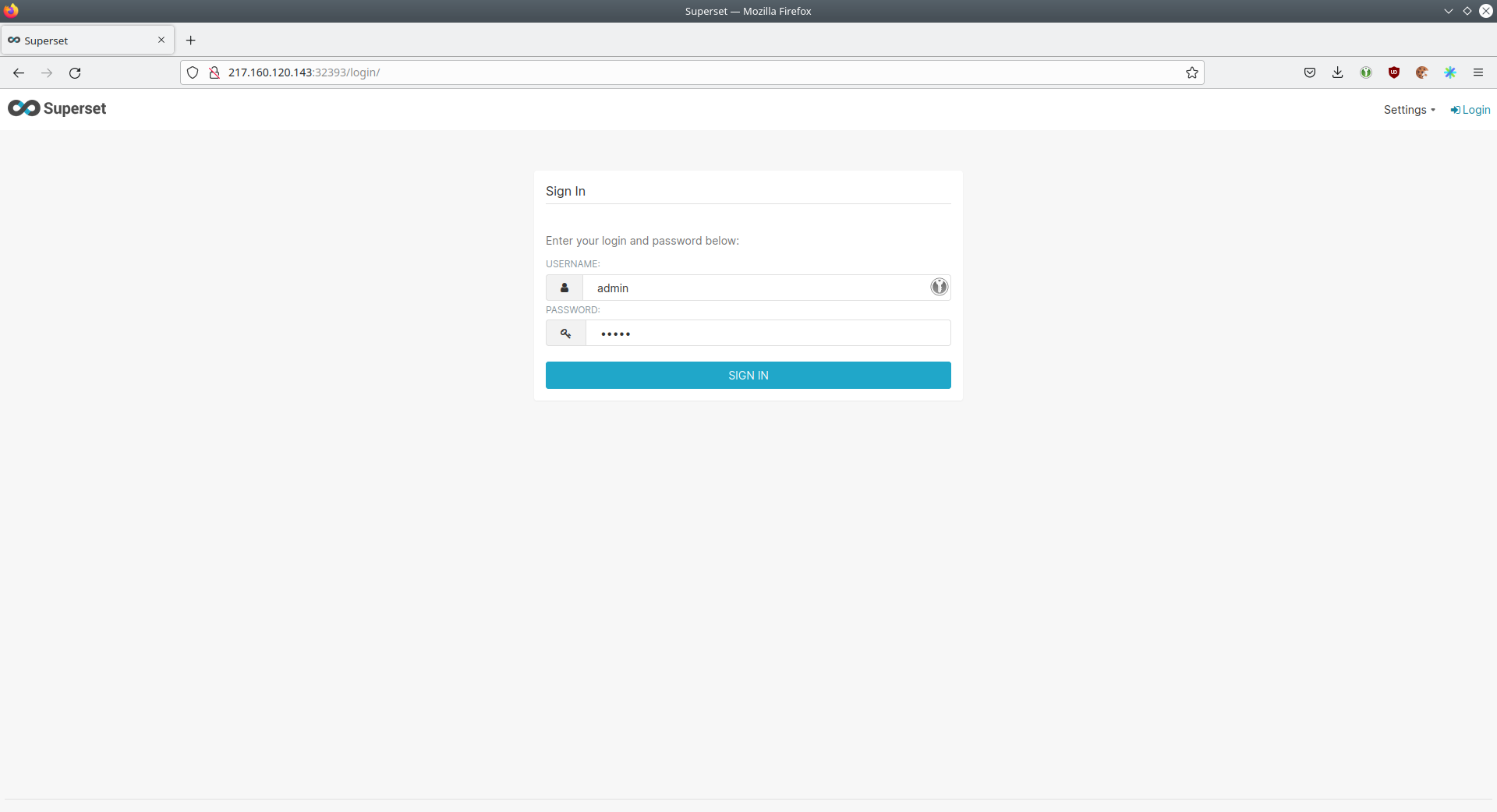
Log in with the username admin and password adminadmin.
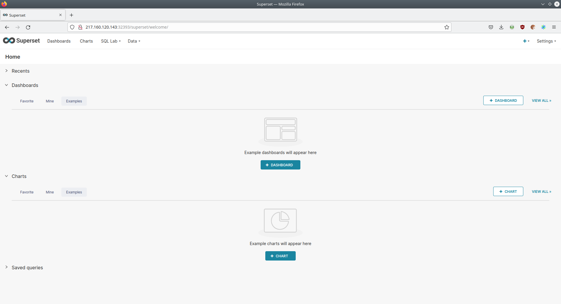
View dashboard
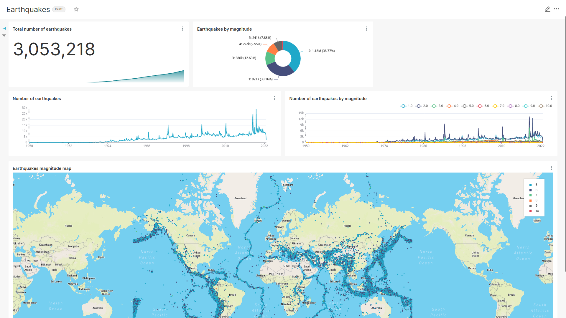
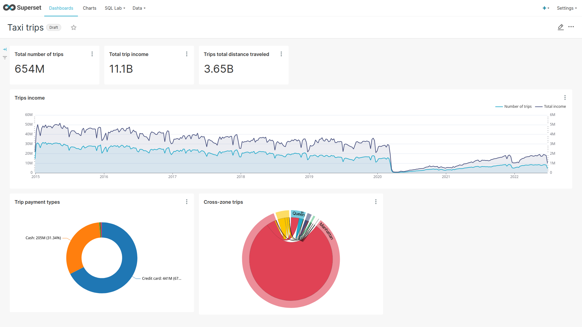
The demo has created dashboards to visualize the different data sources.
To the dashboards click on the tab Dashboards at the top.
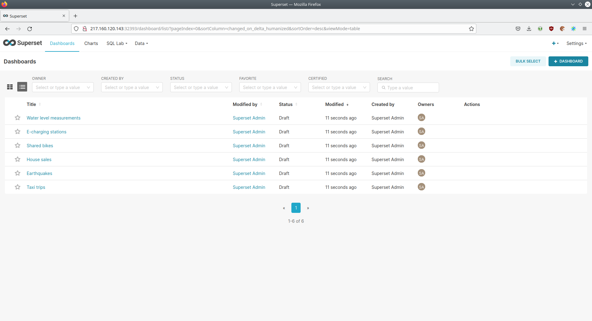
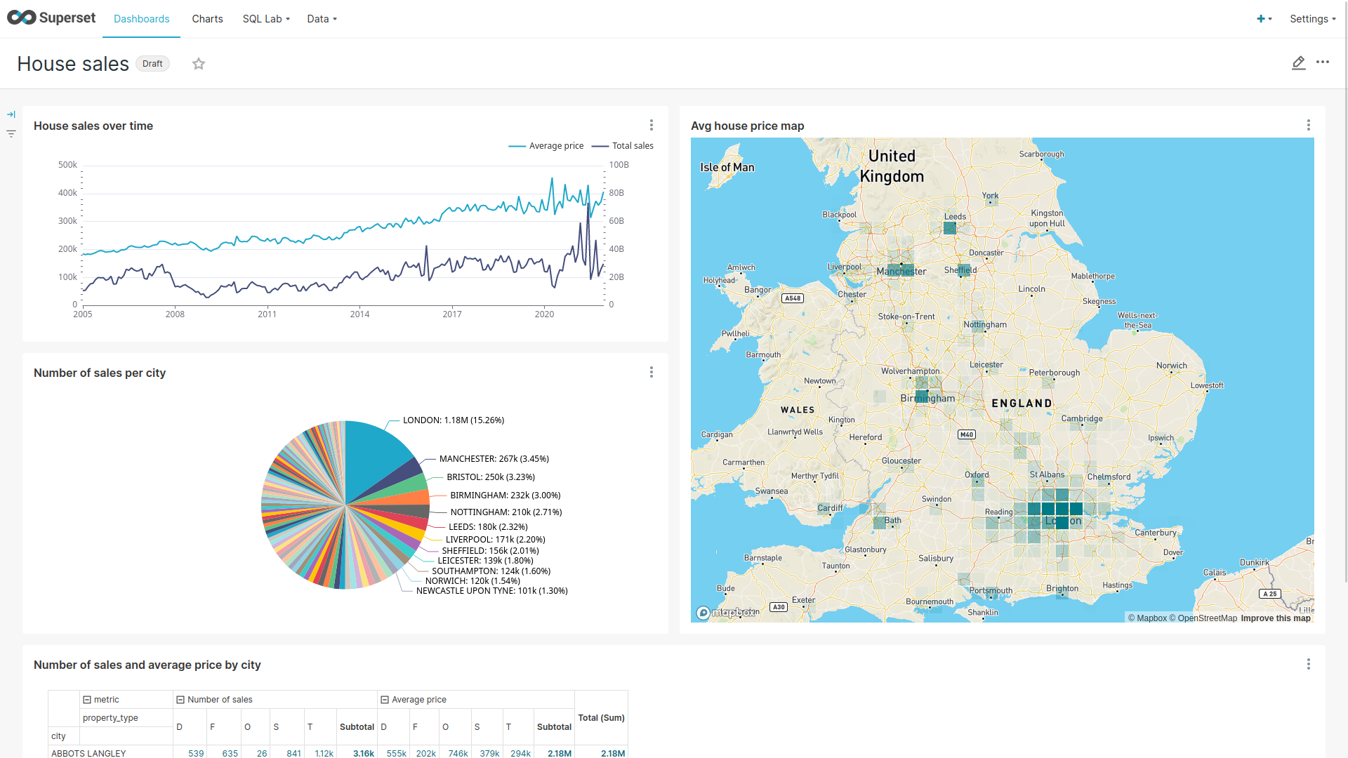
Click on the dashboard called House sales.
It might take some time until the dashboards renders all the included charts.
Another dashboard to look at is Earthquakes.
Another dashboard to look at is Taxi trips.
There are multiple other dashboards you can explore on you own.
View charts
The dashboards consists of multiple charts.
To list the charts click on the tab Charts at the top.
Execute arbitrary SQL statements
Within Superset you can not only create dashboards but also run arbitrary SQL statements.
On the top click on the tab SQL Lab → SQL Editor.
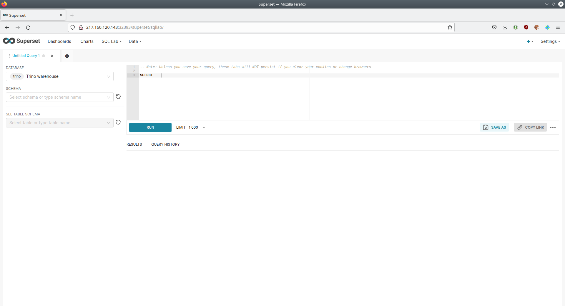
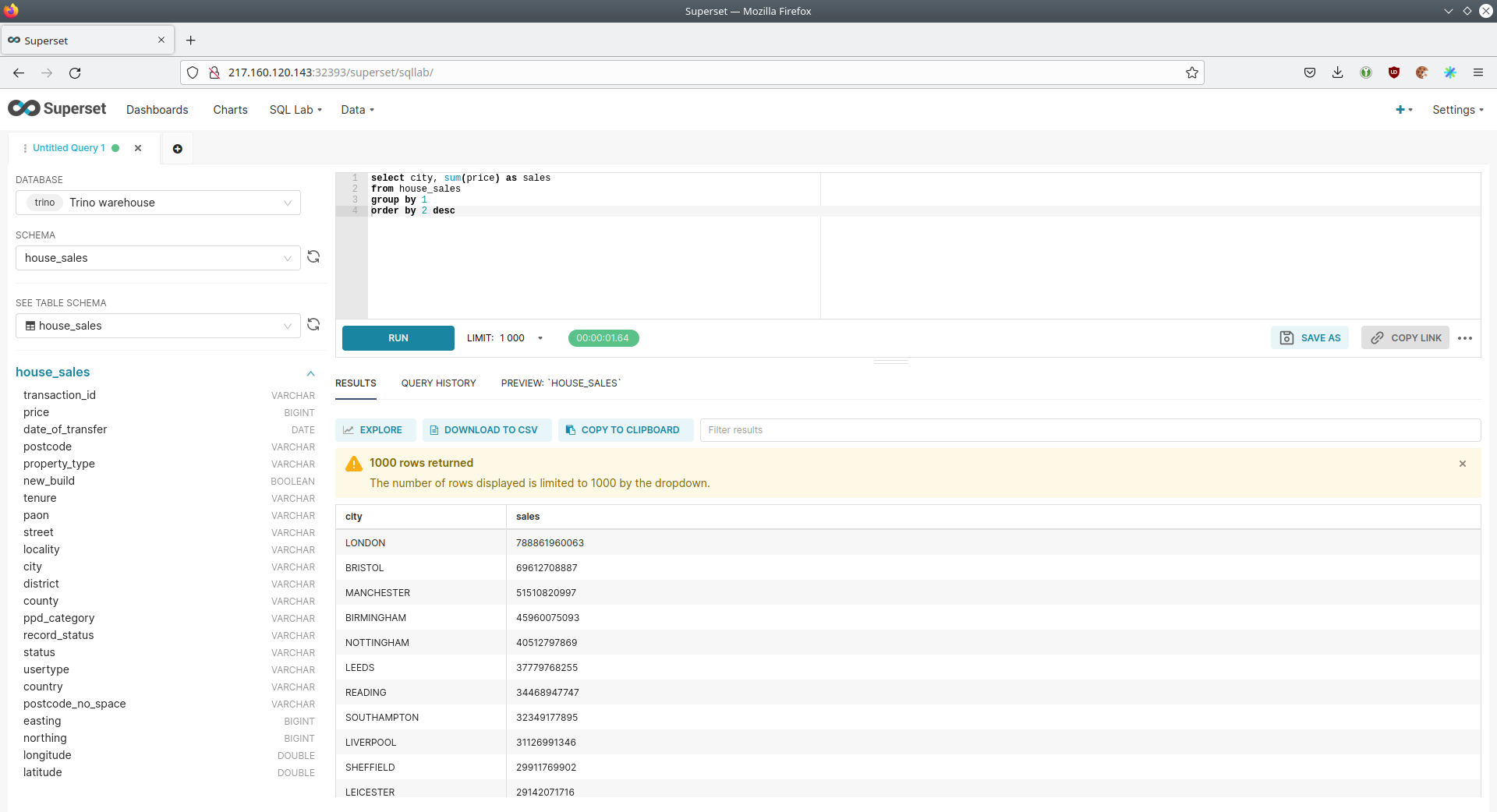
On the left select the database Trino lakehouse, the schema house_sales and set See table schema to house_sales.
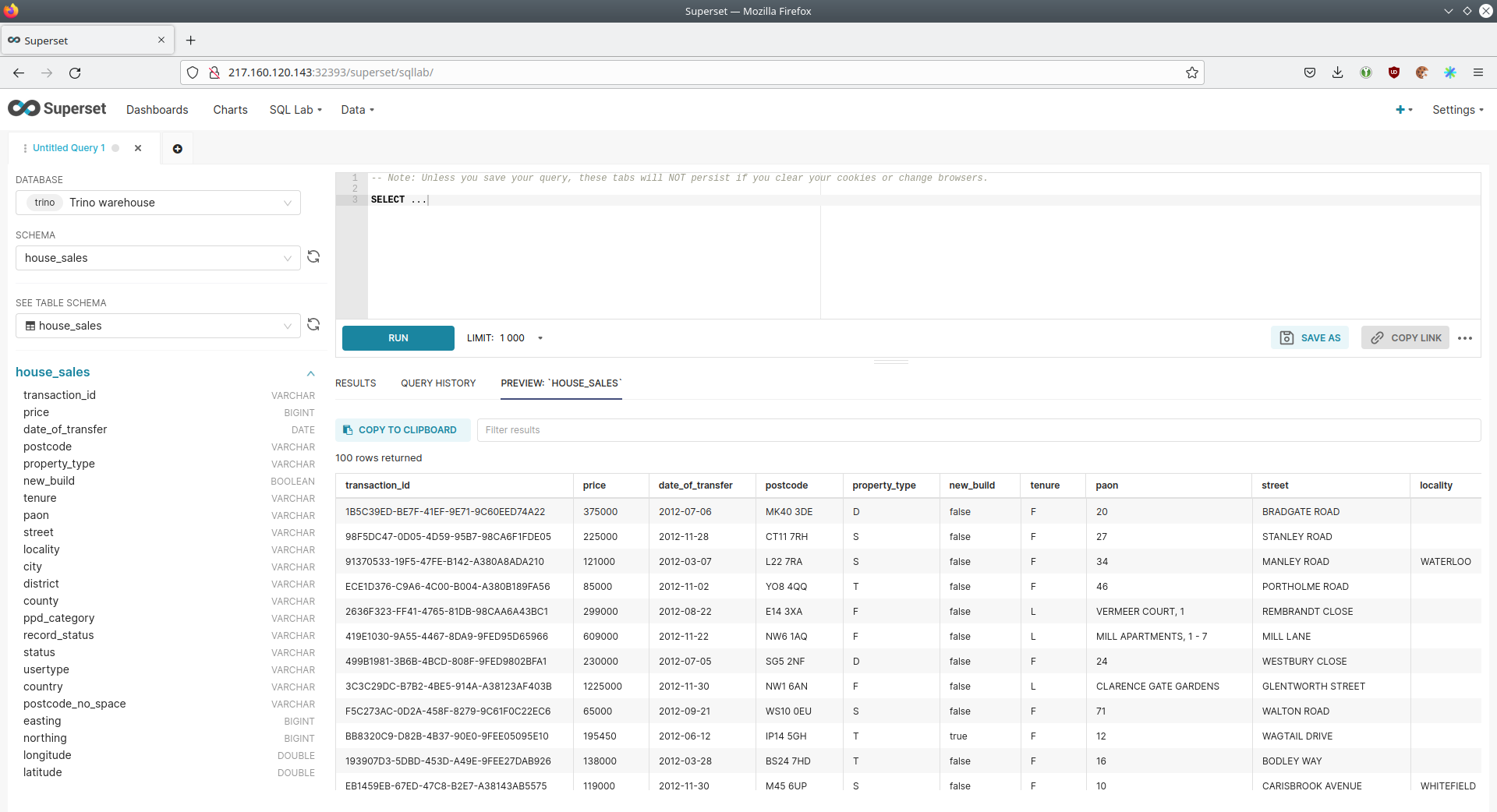
On the right textbox enter the desired SQL statement. If you do not want to make one up, you can use the following:
select city, sum(price) as sales
from house_sales
group by 1
order by 2 desc